Preface
This article records my study of the SVM algorithm in machine learning. It introduces SVM principles and simple applications, using hands-on experiments to build an understanding of SVM.
I. Introduction
1.1 What Is Machine Learning?
Machine learning has no single authoritative definition, but the field's pioneer Arthur Samuel informally defined it as a field of study that gives computers the ability to learn without being explicitly programmed for the problem.
We can therefore think of machine learning as the study of how computer programs automatically improve their performance as they gain experience.
1.2 Classification Algorithms
Classification is an important technique in both data mining and machine learning, with applications throughout society. A classification task learns a target function—usually called a classification model or classifier—that maps each attribute set to a predefined class label. Both classification and regression can predict outcomes, but classification labels are discrete, whereas the target attribute in regression-based predictive modeling is continuous.
Building a classifier generally has two stages: training and testing. Before constructing the model, the dataset is randomly divided into training and test sets. During training, the attributes of the training data are analyzed to produce a description or model for each attribute. During testing, that model classifies the test set and its accuracy is measured. Testing is generally far less expensive than training.
To improve classification accuracy, effectiveness, and scalability, data is usually preprocessed before classification, including:
(1) Data cleaning. Its purpose is to eliminate or reduce noise and handle missing values.
(2) Relevance analysis. Many attributes in a dataset may be unrelated to the classification task; including them can slow or mislead learning. Relevance analysis removes these irrelevant or redundant attributes.
(3) Data transformation. Data can be generalized to higher-level concepts. For example, the continuous attribute "income" can be generalized into the discrete values low, medium, and high, while the nominal attribute "city" can be generalized to the higher-level concept "province." Data can also be normalized, scaling an attribute's values into a smaller interval such as [0, 1].
Classification models can be constructed using decision trees, rule-based methods, nearest neighbors, Bayesian methods, artificial neural networks, and other approaches.
II. Support Vector Machines
2.1 Basic SVM Concepts
A support vector machine (SVM) is a binary classification model. Its basic form is a linear classifier with the maximum margin in feature space; its learning strategy maximizes that margin and ultimately reduces to solving a convex quadratic-programming problem.
2.2 The Basic Idea of SVM
SVM can be understood in two parts.
First, what is a support vector? Put simply, it is a vector point that supports the hyperplane separating two classes.
Second, what does "machine" mean here? The machine is an algorithm. In machine learning, algorithms are often treated as machines—for example, a classification machine, also called a classifier. A support vector machine is a supervised-learning method widely used for statistical classification and regression analysis.
Support vector machines emerged in the mid-1990s as a machine-learning method based on statistical learning theory. By seeking to minimize structural risk, they improve generalization and minimize both empirical risk and the confidence interval, allowing useful statistical regularities to be learned even from relatively small samples.
We can understand the basic idea of SVM through several examples.
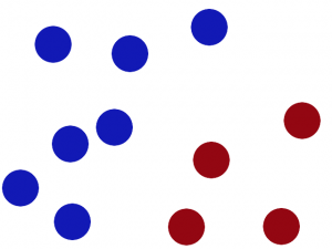
Figure 2.1 contains balls in two colors that need to be separated by a line, as shown in Figure 2.2.
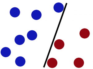
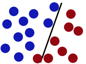
This seems straightforward, but after adding more balls the same line may no longer work well, as Figure 2.3 shows.
This is where SVM is useful. It places the line in the best position so that the space on either side is as large as possible, as shown in Figures 2.4 and 2.5.
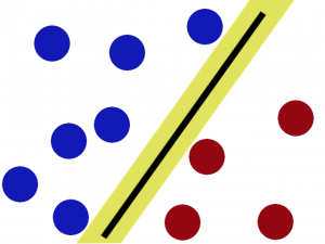
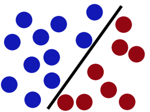
Even if more balls are added, this line remains in the best position. But the SVM idea goes further: what if the blue and red balls are mixed, as in Figure 2.6?
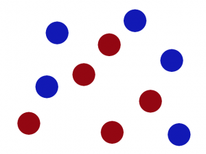
Here we can use an important SVM trick: imagine lifting the diagram into space while looking down from above. A surface analogous to the earlier line must then exist, as shown in Figure 2.7.
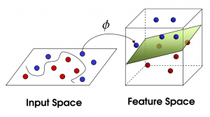
After this surface appears, looking down from above produces the view shown in Figure 2.8.
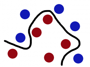
At this point we can translate the example into SVM terminology. The balls are the data, the line is the classifier, maximizing the gap is the optimization objective, lifting the problem into another space is kernelling, and the surface is the hyperplane.
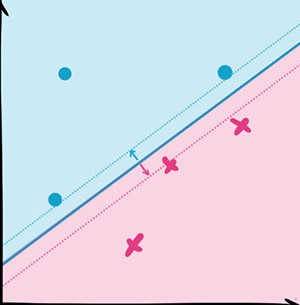
As Figure 2.9 shows, the core idea of SVM is to find a decision boundary between different classes so that samples fall on opposite sides and remain as far from the boundary as possible. The earliest SVMs used flat planes and were quite limited. Kernel functions let us map a plane into a curved surface, greatly expanding the range of problems to which SVM can be applied.
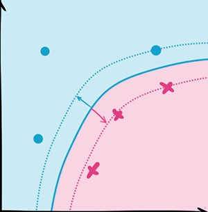
The improved SVM was likewise adopted widely and demonstrated excellent accuracy in real classification tasks.
2.3 Common SVM Models
Common SVM models fall into two categories: linear and nonlinear support vector machines. This article focuses on the soft-margin maximization model for linear SVMs. Before introducing it, we first need to understand support vectors and the objective function of an SVM model.
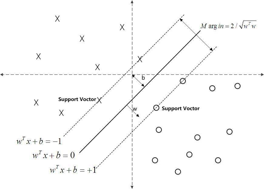
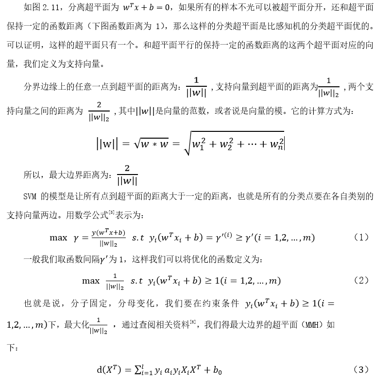
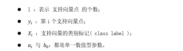
The symbols in the formula mean:
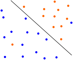
For a test instance, substitute its values into the preceding formula and classify it according to the sign of the result. Linear SVMs can encounter cases where a small number of outliers make an otherwise linear dataset no longer linearly separable, as shown in Figure 2.12.
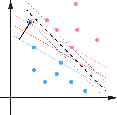
Another situation is not completely inseparable but can still seriously harm the model's generalization. In Figure 2.13, if the outlier were ignored, the SVM hyperplane would be the red line. A single blue outlier instead causes the learned hyperplane to become the thick dashed line, severely affecting the classification model's predictions.
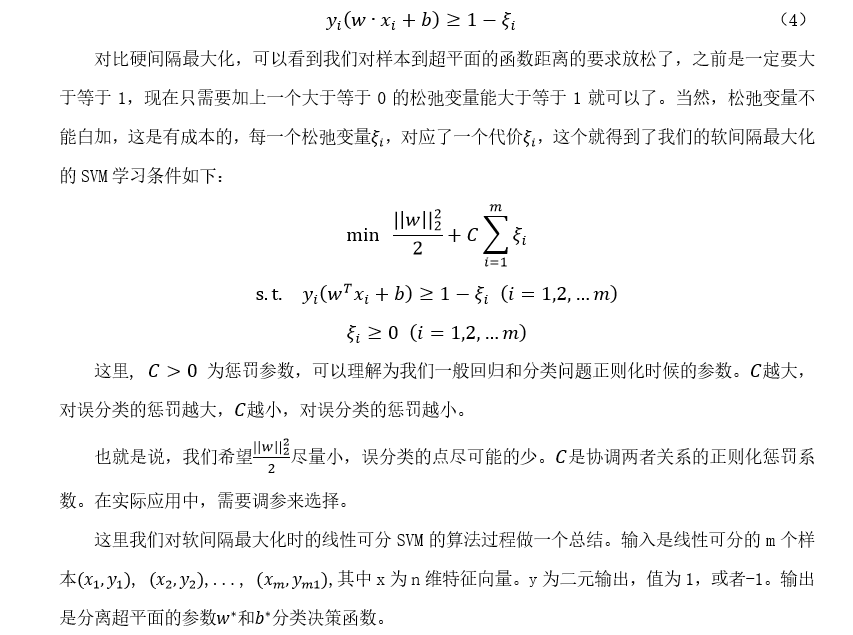
This is precisely why SVM introduces soft-margin maximization. The soft margin7is defined in contrast to a hard margin. We can regard Equation (2) above as the condition for maximizing a hard margin. For every sample (x_i, y_i) in the training set, SVM introduces a slack variable ξ_i ≥ 0, making the functional margin plus the slack variable at least 1. In other words:
The soft margin is easier to understand if we view it spatially. The situation in Figure 2.12 can be handled in two steps:
Use a nonlinear mapping to transform the vector points in the original dataset into a higher-dimensional space. In that higher-dimensional space, find a linear hyperplane that separates them.
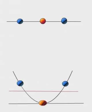
As shown in Figure 2.14, map the problem from one dimension into two and solve it in the two-dimensional space.
III. Applications of Support Vector Machines
3.1 Visualizing the Model
In this example, we primarily use Python's sklearn library to draw and visualize the hyperplane.
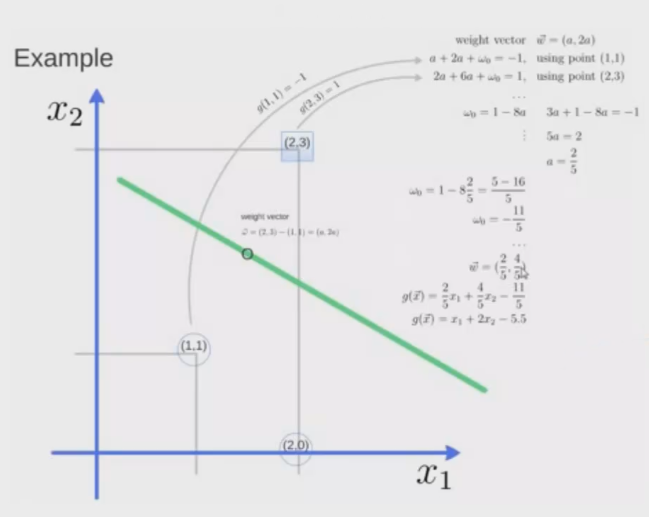
Figure 3.1 contains three points in two-dimensional space: (1, 1), (2, 0), and (2, 3). The first two belong to one class and the third to another. Two of the points, (1, 1) and (2, 3), are support vectors. The support_vectors_ property in sklearn returns the exact points; the programming example is shown in Figure 3.2.
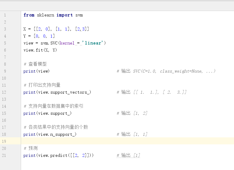
The output is shown in Figure 3.3.
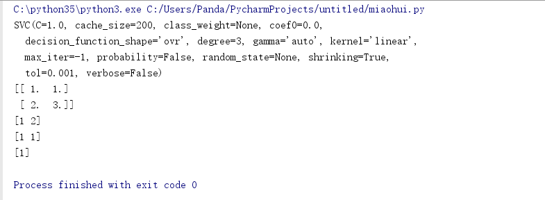
Because there is one support vector on each side of the boundary, view.n_support_ returns [1, 1]. Similarly, we can increase the number of points and draw the hyperplane for visualization. The steps are as follows:
Construct the model Collect the data Select points and find the target line Plot the result
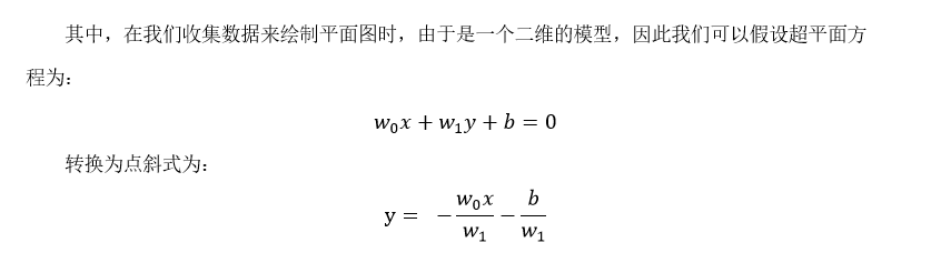
The programming example is shown in Figure 3.4.
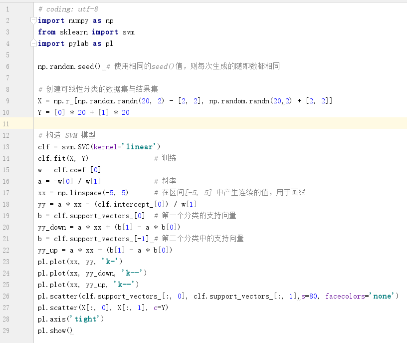
# coding: utf-8
import numpy as np
from sklearn import svm
import pylab as pl

np.random.seed() # with the same seed() value the same random numbers are produced every time

# build a linearly separable dataset and its labels
X = np.r_[np.random.randn(20, 2) - [2, 2], np.random.randn(20,2) + [2, 2]]
Y = [0] * 20 + [1] * 20

# build the SVM model
clf = svm.SVC(kernel='linear')
clf.fit(X, Y)                # train
w = clf.coef_[0]
a = -w[0] / w[1]             # slope
xx = np.linspace(-5, 5)      # continuous values over [-5, 5], used to draw the line
yy = a * xx - (clf.intercept_[0]) / w[1]
b = clf.support_vectors_[0]  # support vector of the first class
yy_down = a * xx + (b[1] - a * b[0])
b = clf.support_vectors_[-1] # support vector of the second class
yy_up = a * xx + (b[1] - a * b[0])
pl.plot(xx, yy, 'k-')
pl.plot(xx, yy_down, 'k--')
pl.plot(xx, yy_up, 'k--')
pl.scatter(clf.support_vectors_[:, 0], clf.support_vectors_[:, 1],s=80, facecolors='none')
pl.scatter(X[:, 0], X[:, 1], c=Y)
pl.axis('tight')
pl.show()
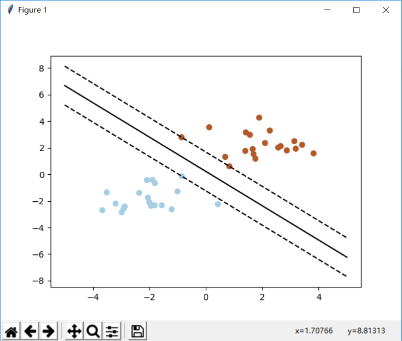
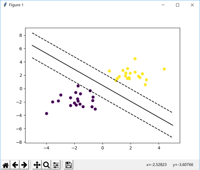
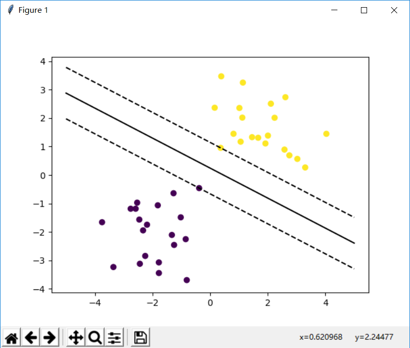
Changing the seed() value lets us plot data with different distributions, as shown in Figures 3.5, 3.6, and 3.7.
3.2 Face Recognition
This algorithm uses principal component analysis (PCA) to reduce the dimensionality of a face dataset and produce several face feature vectors. Each face sample is projected onto those vectors, and the resulting projection coefficients represent the face's features. A support vector machine then classifies the different coefficient vectors to recognize faces.
The main steps are:
(1) Basic information about the face dataset
This test uses the AT&T face dataset from the University of Cambridge. The dataset is 4.68 MB and contains 40 classes, with ten images of the same person in each class.
(2) Splitting the training and test sets
We first load the dataset, flatten each image into a column, and form a data matrix of shape (112×92, 400). We save the face label for each column along with the original image height and width so the images can be reconstructed for display. Splitting the dataset into training and test sets avoids finding separate test images, and because the separated data already includes labels, it also makes prediction results easy to compare with the ground truth.
The train_test_split function provided by sklearn can perform this split:
X_train, X_test, Y_train, Y_test = train_test_split(X, Y, test_size=0.25)
This function returns four results: training-set feature vectors, test-set feature vectors, training labels, and test labels.
(3) Feature dimensionality reduction
The original feature vectors are extremely high-dimensional—1,859 dimensions—which makes model training very complex. Dimensionality reduction is therefore needed to improve performance. Reduced data can sometimes even improve accuracy by decreasing the effect of noise.
(4) Extracting feature points
Extract feature points from the faces for subsequent image visualization.
(5) Constructing the SVM classifier
Because we do not know which parameters will produce the best result, we train with different parameter values and select the best model. After trying multiple values, we search for the model with the highest accuracy.
(6) Prediction
Identify which predictions are correct and which are wrong.
(7) Visualizing the test results
Display the test results, showing the correct identity of each original image and the predicted identity.
The main example code used in this test is shown below:
from __future__ import print_function
from time import time
import logging
import matplotlib.pyplot as plt
import cv2
from numpy import *
from sklearn.model_selection import train_test_split
from sklearn.model_selection import GridSearchCV
from sklearn.metrics import classification_report
from sklearn.metrics import confusion_matrix
from sklearn.decomposition import PCA
from sklearn.svm import SVC

# read the images
PICTURE_PATH = "F:\\face\\"
def get_Image():
    for i in range(1,41):
        for j in range(1,11):
            path = PICTURE_PATH + "\\s" + str(i) + "\\"+ str(j) + ".pgm"
            img = cv2.imread(path)
            img_gray = cv2.cvtColor(img, cv2.COLOR_BGR2GRAY)
            h,w = img_gray.shape
            img_col = img_gray.reshape(h*w)
            all_data_set.append(img_col)
            all_data_label.append(i)
    return h,w

all_data_set = []
all_data_label = []
h,w = get_Image()

X = array(all_data_set)
y = array(all_data_label)
n_samples,n_features = X.shape
n_classes = len(unique(y))
target_names = []
for i in range(1,41):
    names = "person" + str(i)
    target_names.append(names)

print("Total dataset size:")
print("n_samples: %d" % n_samples)
print("n_features: %d" % n_features)
print("n_classes: %d" % n_classes)

# split into training and test sets
X_train, X_test, y_train, y_test = train_test_split(
    X, y, test_size=0.25, random_state=42)
# dimensionality reduction
n_components = 20
print("Extracting the top %d eigenfaces from %d faces"% (n_components, X_train.shape[0]))
t0 = time()
pca = PCA(n_components=n_components, svd_solver='randomized',whiten=True).fit(X_train) # pick an SVD solver
print("done in %0.3fs" % (time() - t0))
eigenfaces = pca.components_.reshape((n_components, h, w))  # eigenfaces
print("Projecting the input data on the eigenfaces orthonormal basis")
t0 = time()
X_train_pca = pca.transform(X_train)  # projection coefficients of the training set
X_test_pca = pca.transform(X_test)    # projection coefficients of the test set
print("done in %0.3fs" % (time() - t0))
print("Fitting the classifier to the training set")
t0 = time()
param_grid = {'C': [1e3, 5e3, 1e4, 5e4, 1e5], 'gamma': [0.0001, 0.0005, 0.001, 0.005, 0.01, 0.1], }
clf = GridSearchCV(SVC(kernel='rbf', class_weight='balanced'), param_grid)
# class_weight='balanced' scales the class weights inversely to class frequency,
# which keeps the model from overfitting an over-represented class
clf = clf.fit(X_train_pca, y_train)
print("done in %0.3fs" % (time() - t0))
print("Best estimator found by grid search:")
print(clf.best_estimator_)

print("Predicting people's names on the test set")
t0 = time()
y_pred = clf.predict(X_test_pca)
print("done in %0.3fs" % (time() - t0))

print(classification_report(y_test, y_pred, target_names=target_names))
print(confusion_matrix(y_test, y_pred, labels=range(n_classes)))

def plot_gallery(images, titles, h, w, n_row=3, n_col=4):
    plt.figure(figsize=(1.8 * n_col, 2.4 * n_row))
    plt.subplots_adjust(bottom=0, left=.01, right=.99, top=.90, hspace=.35)
    for i in range(n_row * n_col):
        plt.subplot(n_row, n_col, i + 1)
        plt.imshow(images[i].reshape((h, w)))
        plt.title(titles[i], size=12)
        plt.xticks(())
        plt.yticks(())
def title(y_pred, y_test, target_names, i):
    pred_name = target_names[y_pred[i]-1]
    true_name = target_names[y_test[i]-1]
    return 'Predicted: %s\nResult:      %s' % (pred_name, true_name)

prediction_titles = [title(y_pred, y_test, target_names, i)for i in range(y_pred.shape[0])]
eigenface_titles = ["Eigenface %d" % i for i in range(eigenfaces.shape[0])]
plot_gallery(X_test, prediction_titles, h, w)
plot_gallery(eigenfaces, eigenface_titles, h, w)
plt.show()
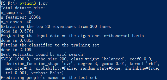
Running the example first produces the projection coefficients of the training and test sets on the feature vectors, together with the SVM classifier, as shown in Figure 3.8.
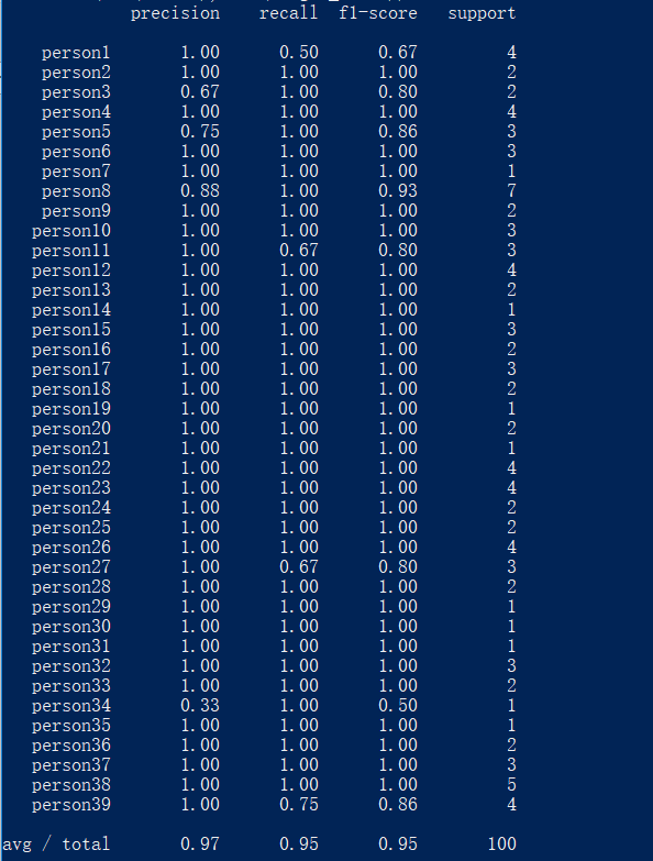
A table containing precision, recall, F1 score, and the number of test samples is also generated, as shown in Figure 3.9.
Finally, we obtain the set of eigenfaces and the prediction results, as shown in Figures 3.10 and 3.11.
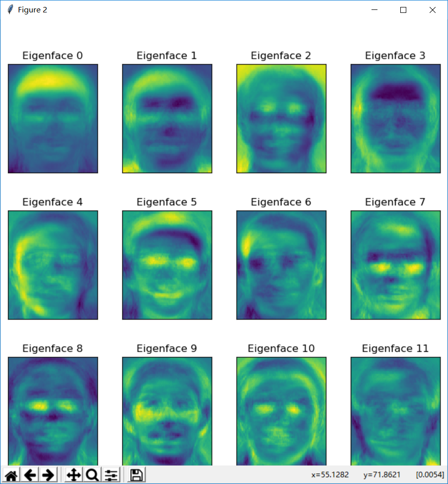
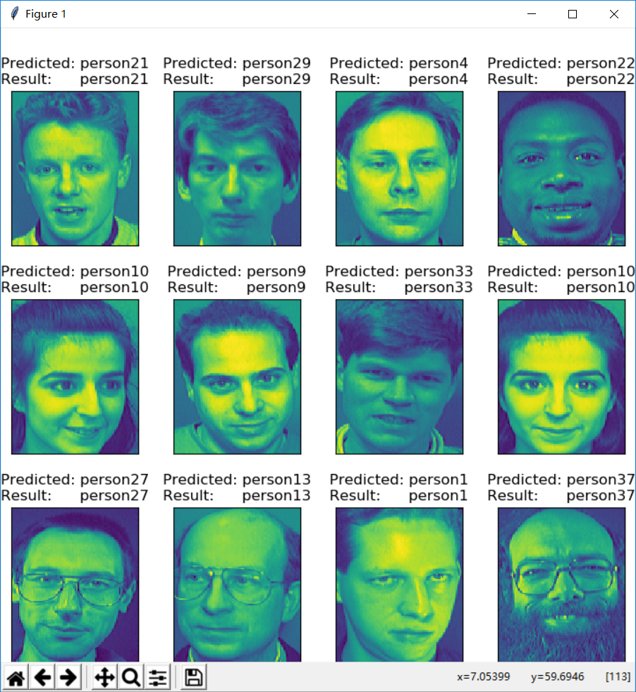
Figure 3.11 shows that most predictions are correct. Figure 3.10 contains eigenfaces abstracted from the feature points. Although this abstract feature extraction is hard for people to recognize, it is very useful to a machine.
IV. Advantages and Disadvantages of SVM
4.1 Advantages of SVM
The main advantages of SVM include:
It is designed specifically for finite samples. Its goal is to obtain the best solution from the information currently available, not merely an optimum approached as the sample size tends toward infinity;
The algorithm ultimately becomes a quadratic optimization problem. In theory, it yields a global optimum, avoiding the local extrema that neural-network methods cannot escape;
The algorithm maps the real problem nonlinearly into a high-dimensional feature space, then constructs a linear discriminant function there to replace the nonlinear function in the original space. This preserves strong generalization while cleverly handling dimensionality: algorithmic complexity does not depend on the number of sample dimensions.
4.1 Disadvantages of SVM
Several difficult problems in current SVM research remain to be solved, including:
There is little theoretical guidance for constructing and choosing kernel functions and their parameters. Kernel choice affects classifier performance, yet theory offers limited help in choosing a suitable kernel and determining its parameters from prior knowledge of the problem and the available samples.
Training on large datasets remains difficult. The conflicts between training speed and sample-set size, and between test speed and the number of support vectors, are still not fully resolved. Effective training and classification algorithms for large sample sets remain an open problem.
Effective algorithms for multiclass classification and optimized multiclass SVM design remain open problems. Algorithms for training multiclass SVMs have been proposed, but efficient multiclass classification and optimal multiclass SVM design still require further research.
IV. Summary
Machine learning includes many other classification algorithms, such as decision trees, rule-based classifiers, Bayesian classifiers, and artificial neural networks.
This article has discussed the support vector machine algorithm. SVM rests on VC-dimension theory and structural risk minimization from statistical learning theory. From finite sample information, it seeks the best tradeoff between model complexity and learning capacity in order to generalize well. It automatically finds support vectors with strong discriminatory power and builds a classifier that maximizes the margin between classes. At the same time, SVM can depend heavily on large training datasets. Obtaining enough training data and reconciling training speed with dataset scale remain practical problems.
In short, SVM has been applied successfully to areas such as face, handwriting, and fingerprint recognition. These applications demonstrate the potential advantages of structured learning methods developed from VC-dimension theory and the principle of structural risk minimization.
Related Download
Link:https://pan.baidu.com/s/1slE7s2h Password: kdn7
References: 1 Liu Hongyan, Chen Jian, and Chen Guoqing. A Survey of Data Classification Algorithms in Data Mining 2 Tao Qing, Cao Jinde, and Sun Demin. A Regression Method Based on Support Vector Classification 3 Luo Haijiao and Liu Xian. Research and Application of Classification Algorithms in Data Mining 4 Iddo. Support Vector Machines explained well 5 Nello Cristianini and John Shawe-Taylor. An Introduction to Support Vector Machines 6 Deng Naiyang and Tian Yingjie. A New Method in Data Mining: Support Vector Machines 7 Hsuan-Tien Lin. Machine Learning Techniques. MOOC 8 Duan Jijun, Chen Lin, Wang Haiyan, and Tian Na. Target Recognition Based on Data-Mining Techniques and Support Vector Machines 9 Zhu Lingyun and Cao Changxiu. Defect Recognition Based on Support Vector Machines 10 Support Vector Machines explained well 11 What Does Support Vector Machine (SVM) Mean? 12 An Accessible Introduction to the SVM Algorithm 13 Classification Algorithms: Support Vector Machines—Applications 14 Scikit-learn Example: PCA + SVM Face Recognition with the AT&T Dataset