The core Transformer architecture has remained largely stable since its introduction. Most iteration has focused on input encoding and pretraining objectives, while the output side has continued to be dominated by autoregressive generation.
In September 2026, two releases put output mechanisms back in focus. On September 15, TypeSafe AI emerged from stealth with the closed-source Jev model and announced a $40 million seed round led by DCVC [1]; on September 18, Nandakishor Mukkunnoth of Convai Innovations open-sourced the Laya model family, including all weights and architectural details [2]. These models retain natural-language understanding but perform no autoregressive token-by-token generation. Once the input has been processed, they emit a probability distribution and act purely as decision engines.
1. Architectural Evolution and the Rise of Decoder-only Models
The original 2017 Transformer [3] contains both an Encoder and a Decoder and was designed for machine translation. Its main advance was the use of self-attention instead of recurrent neural networks.
Self-Attention: Each token produces Query, Key, and Value vectors. Its Query is dotted with every position's Key to obtain weights, and the Values are combined using those weights. All positions can be computed in parallel, unlike an RNN, which must advance sequentially through time steps.
Attention Mask: Before Softmax, positions that must remain invisible are assigned negative infinity in the attention scores. The mask determines which sequence positions each token can see and is the fundamental distinction among the three architectures.
The architecture later split into three main forms:
- BERT [4] is a representative Encoder-only model, with bidirectional attention, suited to text classification, information retrieval, and content moderation;
- T5 [5] is a representative Encoder-Decoder model, suited to sequence-mapping tasks such as translation and summarization;
- GPT [6] is a representative Decoder-only model, with causal attention and autoregressive next-token prediction.
The essential differences lie in what each attention mask makes visible and where the training loss is computed.
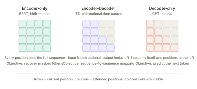
Decoder-only eventually became the dominant architecture for general-purpose language models because several engineering and training advantages reinforce one another. BigScience evaluated these effects systematically in its comparison of architectures and pretraining objectives [7].
Training-signal density. Every token in an autoregressive sequence contributes to the loss. A masked language model computes loss only over masked positions; BERT originally masks about 15% of tokens, so the same corpus supplies far fewer gradient signals.
A unified interface. Question answering, code generation, reasoning, and multi-turn dialogue can all be reduced to continuing a text sequence, so each task does not need a separate output head.
KV Cache compatibility. Causal attention ensures that later tokens cannot rewrite the representations of tokens already generated, so those representations can be cached and reused.
KV Cache: Attention needs the Key and Value from every previous position. Under a causal mask, the K/V for token n does not depend on later tokens, so it can be computed once and cached. Generation of token n+1 reads that cache, reducing the work per step from O(n²) to O(n). Bidirectional attention cannot do this, because adding a token changes the representations of all earlier tokens. This is one reason Encoder-only models are poorly suited to long-form generation.
2. The Latency Cost of Autoregression
Large-model inference has two phases.
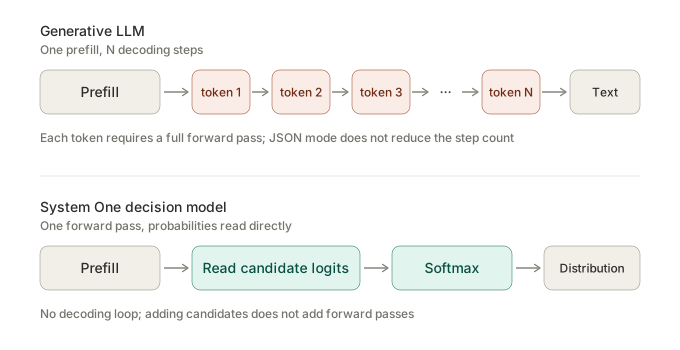
Prefill: The complete prompt is processed in parallel. One forward pass creates the model's internal representation of the input and the corresponding KV Cache. This phase is compute-bound and achieves high GPU utilization.
Decode: The model generates one token at a time. Each token requires another complete forward pass before the new token is appended to the context. This phase is memory-bound: at every step, the full model weights must be moved from GPU memory into the compute units to produce a single token.
The bottleneck is straightforward: even if the model has formed a complete internal representation of the problem by the end of Prefill, an autoregressive pipeline must still write the answer one token at a time. Post-training chain-of-thought reasoning (as in DeepSeek-R1 [8]), makes the model generate substantial reasoning before reaching a conclusion. Reasoning improves, but token consumption and latency rise with it.
Recent architectural optimizations, including Mixture of Experts (MoE [9]) and techniques that compress attention or KV Cache, mainly reduceeach step's computation and memory cost; they do not remove token-by-token generation itself.
3. Jev's Non-Generative Output
Jev changes the output mechanism. It does not provide open-ended text chat; its interface exposes only three decision primitives [10]:
- Choice: Selects one item from a caller-defined set of up to 255 options and returns a probability for each option plus a confidence value describing how concentrated the distribution is;
- Score: Scores an item on a two-to-ten-level ordinal scale described in natural language and returns a probability-weighted position, which may fall between two levels;
- Noul: Estimates the probability that a statement is true and returns a value from 0 to 1.
The API uses one endpoint. The caller supplies a state, as text or JSON, and a set of named questions. The model returns numeric probabilities—for example, percentages for routing a ticket to technical, billing, or sales—with no explanatory text.
This is different from structured output in a large language model (JSON Mode). A general-purpose LLM in JSON mode still runs a token-by-token Decode loop. Constrained decoding only narrows the sampling space to legal braces, field names, and formatting characters. It does not remove any generation steps; it only reduces the chance of a parsing failure.
After Prefill, Jev reads the probability assigned to each option directly from the final layer's hidden state and skips decoding. The company reports end-to-end latency of 70 to 500 milliseconds, a price of $0.042 per million input tokens with no output charge, and a 40× to 200× speed advantage over frontier LLMs on comparable tasks [11]. One third-party test measured response times between 236 and 276 milliseconds [12].
Why the absence of hallucination is structural: The output space is limited to the candidate set declared in advance. The model cannot return a value outside that set or produce an invalid format. This is type safety enforced by the interface, not behavior learned during training. The cost is that the model can answer only the question it was given; it cannot volunteer a fourth possibility that the caller failed to consider.
4. Probability Calibration: The Practical Value of Decision Models
A model can be 95% accurate and still be difficult to route safely if its confidence scores are unreliable: the system cannot tell which 95% to trust.
Calibration: Among samples assigned 0.9 confidence, the observed accuracy should be close to 90%. Common measurements include ECE (Expected Calibration Error, which bins predictions by confidence and takes the weighted mean of the gap between confidence and observed accuracy in each bin) and Brier score (the mean squared error between predicted probabilities and true labels). Guo et al. showed in 2017 that modern deep networks are generally overconfident, with the effect becoming more pronounced as models grow; temperature scaling (dividing logits by a scalar T before Softmax) is the simplest effective post-hoc calibration method [13].
Once probabilities are calibrated, application code can route by numeric thresholds: execute automatically above 0.95, trigger a second check between 0.7 and 0.95, and send cases below 0.7 to a human.
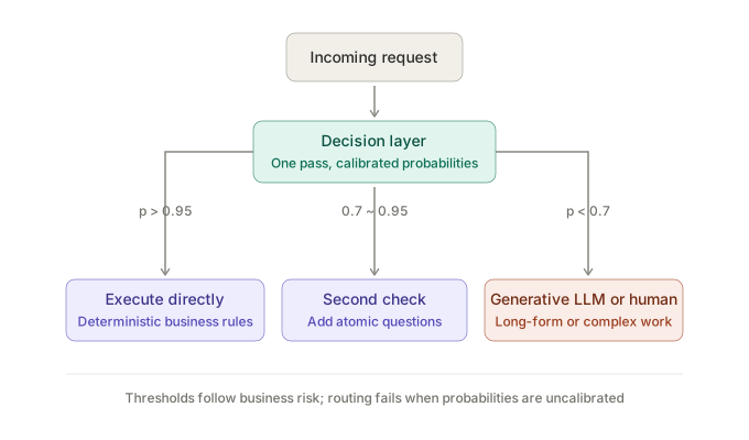
Laya's published data shows the practical difficulty of calibration. The base checkpoint has a raw ECE of 0.213 without temperature scaling; fitting a domain-specific temperature reduces it to 0.081 [14]. Reading raw probabilities from a model is therefore insufficient; the temperature must be fitted again on the deployment data distribution.
This mechanism works well when a complex business judgment can be split into independent atomic questions. For phishing detection, instead of asking whether an entire message is malicious, the system can ask whether the sender matches the domain, whether the body requests credentials, whether it creates urgency, and whether links conceal redirects. Each question returns a probability, and program control flow combines the results. Software owns deterministic business rules; the model handles narrow, ambiguous classifications.
5. How This Differs from a Traditional Classifier, and How Laya Works
Producing class probabilities in one forward pass resembles a traditional BERT classifier. The difference is where the task is defined.
A traditional BERT classifier stores its task in the model parameters: a spam model detects only spam, a sentiment model detects only sentiment, and the number of classes is fixed by the output-head dimension during training. A new use case needs new data and fine-tuning. Jev-style models put the question, background state, and candidates in the input text, allowing the classification task itself to be interpreted at inference time.
The open-source Laya model [2: 1] provides a clear implementation reference. It is based on ModernBERT-large [15] (421 million parameters, English) and the multilingual mmBERT-base (322 million parameters). Both use an Encoder-only architecture and are licensed under Apache-2.0.
The implementation concatenates the background information, question, and candidates into one input. It assigns a separate [MASK] position to each candidate option, produces logits for all options in one forward pass, and normalizes them into a probability distribution with Softmax. No text is generated. On a T4 GPU, one question takes 33 milliseconds; in a batch, each question takes 7.2 milliseconds [2: 2]. It also includes a sub-millisecond pure-Python router that uses Unicode script detection to select the English or multilingual checkpoint.
The training method is RLCD (Reinforcement Learning for Calibrated Decisions), the name TypeSafe used for its in-house method in the company's announcement [1: 1], and Laya uses the same term.
Strictly Proper Scoring Rule: A class of reward functions whose expected value is maximized only when the reported probability equals the model's true posterior belief. Logarithmic score, spherical score, and Ranked Probability Score (RPS) for ordered outcomes all belong to this class. Used as an RL reward, such a rule makes overstated confidence mathematically costly, so confidence falls when the model is uncertain. It addresses overconfidence in the training objective rather than repairing it later with temperature scaling [16].
Laya's high accuracy depends on downstream fine-tuning. Its base checkpoints perform close to random selection in the zero-shot typed-decisions benchmark: 0.362 for English and 0.352 for multilingual, compared with a random baseline of 0.318 and a majority-class baseline of 0.461 [14: 1][17]. The widely quoted accuracy of 0.766 comes from a specialized checkpoint fine-tuned on that benchmark's own training set [16: 1]. The official model card is explicit: Laya is a base for rapid specialization, not a zero-shot model.
The option count is also constrained. Candidates share a fixed 256-token head budget, and the recommendation is to keep the list below 20 options. With a larger label space, each label receives too few tokens and accuracy falls sharply [17: 1].
The hard part is not attaching a decision head to a Transformer; that structure is straightforward to implement. The real threshold is general-purpose understanding: reliably understanding a classification task in any domain from a natural-language description, without task-specific fine-tuning. Encoders with three to four hundred million parameters have limited capacity here. Jev has not disclosed its architecture or parameter count, but its zero-shot performance suggests a substantially larger base model.
The Jev-Laya comparison therefore needs qualification. Laya's model card notes that the Jev figures come from public third-party data rather than tests in the same environment; sample sizes and prompts differ. Laya also trails on the soft-probability matching metric, 0.471 versus 0.580. Its argmax is more accurate, but the shape of its probability distribution matches the teacher distribution less closely than Jev's [14: 2][16: 2].
6. Where These Models Fit in a System
The most useful architectural role for this class of non-generative model is a router at the front of the pipeline: it handles initial filtering, intent routing, and risk scoring. Software executes high-confidence requests directly; only low-confidence cases, or tasks that require long-form writing and complex reasoning, go to a generative LLM downstream.
For security systems, this layering also separates judgment from expression. The decision layer emits an auditable number rather than natural language that must be parsed. A rule engine can consume it, thresholds can change with the threat environment, and false positives can be measured and regression-tested. This is more reliable than asking a generative model in a prompt to output only yes or no.
Over the past two years, many teams have applied generative LLMs to every available problem because their generalization made prototypes easy. Even simple classification and routing tasks have been handed to models with tens of billions of parameters, which then decode a {"result": "pass"} JSON object one token at a time. This is convenient during prototyping but produces low throughput, variable latency, and substantial GPU-memory waste in high-concurrency production systems.
The direction taken by Jev and Laya indicates that monolithic LLMs are beginning to give way to layered, decoupled production systems:
-
System 1 and System 2 become separate infrastructure components.
Autoregressive decoding and chain-of-thought reasoning suit complex work such as long-horizon reasoning, coding, and open-ended generation (System 2). Single-pass models focus on perception, classification, and confidence estimation (System 1). Moving intent routing and deterministic decisions to the front of the pipeline removes substantial decoding overhead and can reduce end-to-end latency by an order of magnitude. -
Evaluation returns to standard statistical measurements.
Generative models are difficult to cover with deterministic unit tests and regression checks. A non-generative decision system can instead use temperature scaling, Expected Calibration Error (ECE), and Brier score as primary measurements. It can then apply numeric thresholds for staged rollout, A/B testing, and statistical blocking in the same way as a conventional risk-control or recommendation system. -
Model selection must account for the limits of a lightweight substitute.
The trade-off is concrete. Closed-source Jev demonstrates strong zero-shot generalization from a larger model, but introduces vendor lock-in and opaque billing. Open models such as Laya, with three to four hundred million parameters, are barely usable from base weights in zero-shot settings. Their practical value lies in rapid specialization for a private domain: it requires a defined feedback loop with domain data, RLCD fine-tuning on that distribution, and temperature fitting.
A more likely production pattern is not one large model handling everything, but small, precise decision heads controlling the flow while larger, deeper generators produce open-ended output. Decision and expression become separate jobs.